Bayesian Regression: Likelihood
The working horse of every Bayesian model is the equation:
\[ posterior \propto likelihood \times prior \]
The likelihood is the likelihood of observing the data, given our current set of weights.
Suppose you have a fixed set of weights \(\vec w\).
For example, you have just initialized your weights by drawing them from a multivariate Gaussian distribution.
Now you want to know how likely it is that the data comes from a model specified by \(\vec w\). It helps to think of \(\vec w\) as your null hypothesis which you want to test. So you ask:
- How likely is it that our null hypothesis is true?
- How likely is it that the data was generated from a model specified by \(\vec w\)?
- How likely is it to observe the things that we have observed under the null hypothesis that the data-generating process is described by \(\vec w\)?
For now, think of the likelihood as a probability. Technically, the likelihood can be a probability, but does not have to be. But this doesn’t change the idea behind it.
Think of the dataset as a series of random events, like coin flips. Suppose you throw a coin 3 times and you observe HEAD, HEAD, TAILS. How likely is it that you see such a sequence under the null hypothesis that the coin is fair? Well, it is the probability to observe HEAD, times the probability to observe HEAD, times the probability to observe TAIL.
\[ Pr(\text{Head}\rightarrow \text{Head}\rightarrow \text{Tails}|\text{fair coin})=0.5\times 0.5 \times 0.5=0.5^3 \]
Think of the results of the coin flips as our targets. The three coin flips correspond to targets \(t_1, t_2, t_3\). And we were looking for
\[ Pr(t_1 \cap t_2 \cap t_3 | \text{fair coin})=Pr(t_1| \text{fair coin})\times Pr(t_2| \text{fair coin}) \times Pr(t_3| \text{fair coin}) \]
We can apply this idea to our scenario. The likelihood of observing the kind of data that we observed under null hypothesis \(\vec w\) is given by:
\[ \begin{aligned} L(D|\vec w) =& \left(\text{probability of observing }t_1 \text{ given }\vec w \right)\\ & \times \left(\text{probability of observing }t_2 \text{ given }\vec w \right) \\ & \ \ \vdots \\ & \times \left(\text{probability of observing }t_N \text{ given }\vec w \right) \\ =& p(t_1|\vec w, \vec x_i, D) \times p(t_2|\vec w, \vec x_i, D) \times \dots p(t_N|\vec w, \vec x_i, D) \\ =& \prod_{i=1}^N p(t_i|\vec w, \vec x_i, D) \\ =& \prod_{i=1}^N \underbrace{N(t_i|\vec w^T\vec x_i, \alpha^{-1})}_{ \text{Gaussian density} } \\ \end{aligned} \]
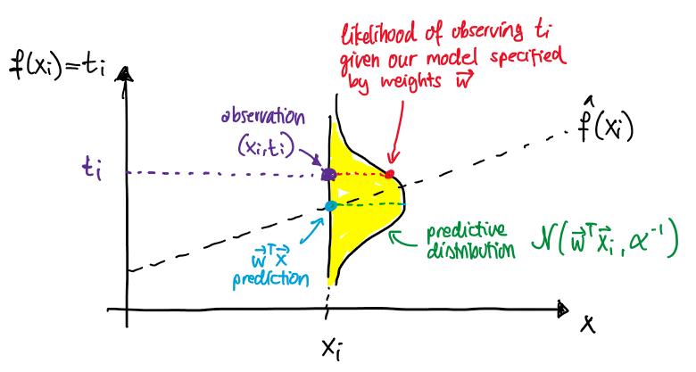
\(N(t_i|\vec w^T \vec x_i, \alpha^{-1}\)) is the density at the point \(t_i\) of the Gaussian distribution with mean \(\vec w^T \vec x_i\) and variance \(\alpha^{-1}\). In R, you would calculate that density with dnorm(x, mean, sd).
The likelihood tells us how likely it is to draw the data that we observed from the distribution \(p(t_i|\vec w, \vec x_i, D)\) for some fixed values of our model parameters \(\vec w\) (and precision \(\alpha\)).
Log-Likelihood
To make things easier, we usually work with the log-likelihood instead of the likelihood:
\[ \begin{aligned} LL(D,\vec w) =& \log L(D|\vec w) \\ =& \log \left(\prod_{i=1}^N p(t_i|\vec w)\right) \\ =& \sum_{i=1}^N \log p(t_i|\vec w) \\ =& \sum_{i=1}^N \log N(t_i|\vec w^T\vec x_i, \alpha^{-1}) \end{aligned} \]
Note that the (log-)likelihood changes if your weights change.
Note: Sometimes people write \(L_{\vec w}(D)\), which you would read as “the likelihood function under the parametrization \(\vec w\)”.
Pseudocode for calculating the log-likelihood
data = data.frame(y = ..., x = ...)
   weights = [0.41, 1.23] # [intercept, slope]
   alpha = 2 # precision of predictive distribution
   loglik = 0
   for i in 1,2,...,N:
       t_i = data$y[i]
       x_i = [1, data$x[i]]
       wTx_i = dot(w, x)
       density_i = normal_density(
           x=t_i,
           mean=wTx_i,
           var=(1/alpha)
       )
       loglik += log(density_i)