Bayesian Regression - Model Setup
Disclaimer: I wrote this primarily for myself. For others, the structure with which I layout the ideas may be less coherent.
Basic Intuition
Non-Bayesian regression gives you a prediction line that tells you the most likely value of the target given some inputs.
Bayesian regression gives you not just a line, but a predictive distribution that tells you how the target is distributed given some inputs.

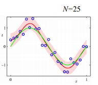
- green line: true underlying function
- red area: graphical representation of the predictive distribution. The narrower the corridor, the less uncertainty there is about where the target value most likely lands.
- red line: the prediction line you get from non-bayesian regression. Note that that line corresponds to the mean of the predictive distribution. The red line represents Maximum Likelihood Estimates.
The predictive distribution tells you how the target is distributed given some input values.
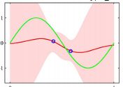
The fewer data points are available, the “broader” our predictive distribution will be, and so the more uncertain we are about our predictions.
In areas with few observations we are less confident about the value of our target. In areas with many observations we are more confident about the value of our target.

Model setup
The predictive distribution
We want to find the predictive distribution \(p(t|\vec w, \vec x,D)\).
The predictive distribution gives me the distribution of our target \(t_i\) given some input vector \(\vec x_i\). The shape of the predictive distribution is specified by weights \(\vec w\), which are calibrated on dataset \(D\).
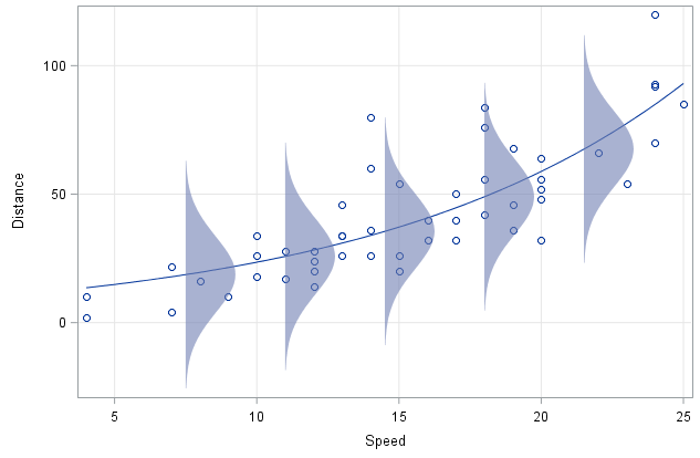
In the figure below you see various \(p(t_i|\vec w, \vec x_i, D)\) for different inputs \(\vec x_i\). The targets were assumed to be normally distributed with mean zero and identical variance. These are common but not obligatory assumptions.

To specify the predictive distribution \(p(t_i|\vec w, \vec x_i, D)\) we make the following assumptions:
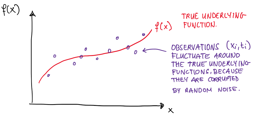
We assume that there is some true underlying function \(f(\vec x)\) that generates the data. Think of some inherent process, a rule of nature, that governs the relationship between input \(\vec x\) and output \(t\).
Unfortunately, wuat we actually observe in nature is often corrupted by randomness. We call this random noise \(\epsilon\). Thus, we never observe \(f(\vec x)\) in the real-world, but a corrupted version \(f(\vec x)+\epsilon\).

Despite random noise being random, it often still has a pattern. That pattern is described by a probability distribution. In many real-world scenarios the underlying pattern is well described by a normal distribution.
\[ t_i = f(\vec x_i) + \epsilon \qquad \text{where} \quad \epsilon \sim N(0,\alpha^{-1}) \]
Intuitively, normally distributed random noise means that
- you most likely observe values around the true value \(f(\vec x_i)\)
- values further away from the true value are less likely
- values to the right and to the left of the true value are equally likely.
In this specification, the observed targets \(t_i\) become a random variable themselves. Thus, they follow a distribution. Because we have chosen normally distributed noise, our targets will be distributed normally:
\[ t_i \overset{\text{iid}}{\sim} N(\vec{w}^T{\vec x_i}, \alpha^{-1}) \]
or
\[ p(t_i|\vec w, \vec x_i, D) = N(t_i|\vec{w}^T{\vec x_i}, \alpha^{-1}) \]
This is the predictive distribution.
Notation of Predictive Distribution in Textbooks
Suppose our model parameters are \(\vec w, \alpha\). These parameters fully specify our predictive distribution:
\[ p(t_n|\vec w, \alpha,\vec x_i, D) \]
Sometimes, textbooks collect all model parameters in another variable \(\theta\). In our case, \(\theta=\{\vec w, \alpha \}\).
The advantage is that we can write our predictive distribution in a simpler way:
\[ p(t_n | \vec w, \theta, D) \]
Sometimes, textbooks also get rid of the \(D\). Recall that the \(D\) indicates that the weights were calibrated on dataset \(D\). This does not need to be the case, for example, when you evaluate the predictive distribution right after randomly initializing the weights. So you also see:
\[ p(t_n | \vec w, \theta) \]
I don’t like it when textbooks “unclutter” notation, but it is how it is. I’ll be more rigorous in my notation, and try to include every variable and parameter that plays a role.